1. What is Reinforcement Learning? 1. 강화학습이란 무엇인가?
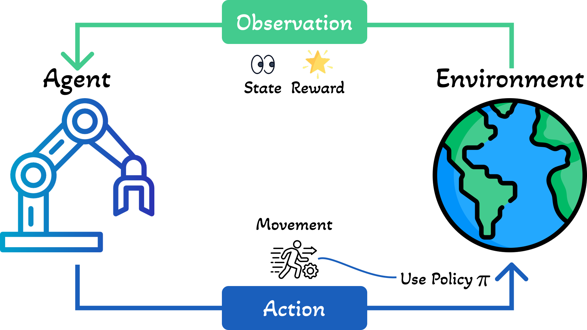
Reinforcement Learning or RL is a class of methods for solving various kinds of sequential decision making tasks. In such tasks, we want to design an agent that interacts with an external environment. The agent maintains an internal state $s_t$, which is passed to its policy $\pi$ to choose an action $a_t = \pi(s_t)$. The environment responds by sending back an observation $o_{t+1}$, which the agent uses to update its internal state using state-update function $s_{t+1}=U(s_t, a_t, o_{t+1})$. See Figure 1 for an illustration.
강화학습(RL)은 다양한 종류의 순차적 의사결정 문제를 해결하기 위한 방법론의 한 종류입니다. 이러한 작업에서는 외부 환경과 상호작용하는 에이전트를 설계하고자 합니다. 에이전트는 내부 상태 $s_t$를 유지하며, 이를 정책 $\pi$에 전달하여 행동 $a_t = \pi(s_t)$를 선택합니다. 환경은 관측값 $o_{t+1}$을 다시 보내며, 에이전트는 이를 사용하여 상태 업데이트 함수 $s_{t+1}=U(s_t, a_t, o_{t+1})$를 통해 내부 상태를 업데이트합니다. 그림 1을 참조하세요.
1.1 Problem Definition 1.1 문제 정의
The fundamental objective of an RL agent is to learn a policy $\pi$ that maximizes the expected cumulative reward. Formally, we define the value function for a policy $\pi$ starting from state $s_0$ as:
RL 에이전트의 근본적인 목표는 기대 누적 보상을 최대화하는 정책 $\pi$를 학습하는 것입니다. 공식적으로, 상태 $s_0$에서 시작하는 정책 $\pi$의 가치 함수를 다음과 같이 정의합니다:
where $s_0$ is the initial state, $R(s_t, a_t)$ is the reward function that measures the immediate value of taking action $a_t$ in state $s_t$, and the expectation is taken over trajectories $\tau = (s_0, a_0, s_1, a_1, \ldots, s_T, a_T)$ generated by following policy $\pi$.
여기서 $s_0$는 초기 상태, $R(s_t, a_t)$는 상태 $s_t$에서 행동 $a_t$를 취했을 때의 즉각적인 가치를 측정하는 보상 함수이며, 기댓값은 정책 $\pi$를 따라 생성된 궤적 $\tau = (s_0, a_0, s_1, a_1, \ldots, s_T, a_T)$에 대해 계산됩니다.
The trajectory distribution is determined by the policy and the environment dynamics:
궤적 분포는 정책과 환경 역학에 의해 결정됩니다:
where $\pi(a_t \mid s_t)$ is the probability of selecting action $a_t$ in state $s_t$ under policy $\pi$, and $p_{\text{env}}(s_{t+1} \mid s_t, a_t)$ is the environment's transition probability distribution (typically unknown to the agent).
여기서 $\pi(a_t \mid s_t)$는 정책 $\pi$ 하에서 상태 $s_t$에서 행동 $a_t$를 선택할 확률이고, $p_{\text{env}}(s_{t+1} \mid s_t, a_t)$는 환경의 전이 확률 분포입니다 (일반적으로 에이전트에게 알려지지 않음).
We define the optimal policy as:
최적 정책을 다음과 같이 정의합니다:
where the expectation is over the initial state distribution $p_0(s_0)$. This formulation embodies the maximum expected utility principle: the agent seeks to maximize its expected long-term reward rather than immediate gains.
여기서 기댓값은 초기 상태 분포 $p_0(s_0)$에 대해 계산됩니다. 이 공식은 최대 기대 효용 원리를 구현합니다: 에이전트는 즉각적인 이득보다는 기대 장기 보상을 최대화하려고 합니다.
Finding the optimal policy is challenging because: (1) the environment dynamics $p_{\text{env}}$ are typically unknown, (2) the state and action spaces can be extremely large or continuous, and (3) we must balance exploration (gathering information) with exploitation (using current knowledge).
최적 정책을 찾는 것은 다음과 같은 이유로 어렵습니다: (1) 환경 역학 $p_{\text{env}}$가 일반적으로 알려지지 않음, (2) 상태 및 행동 공간이 매우 크거나 연속적일 수 있음, (3) 탐색(정보 수집)과 활용(현재 지식 사용) 사이의 균형을 맞춰야 함.
1.2 Episodic vs Continuing Tasks 1.2 에피소드 작업과 연속 작업
If the agent can potentially interact with the environment forever, we call it a continuing task. Alternatively, the agent is in an episodic task, if its interaction terminates once the system enters a terminal state or absorbing state, which is a state which transitions to itself with 0 reward. After entering a terminal state, we may start a new episode from a new initial world state $s_0 \sim p_0$. (The agent will typically also reinitialize its own internal state $s_0$.)
에이전트가 환경과 잠재적으로 영원히 상호작용할 수 있다면, 이를 연속 작업이라고 합니다. 또는, 시스템이 종료 상태 또는 흡수 상태에 진입하면 상호작용이 종료되는 경우 에이전트는 에피소드 작업에 있습니다. 흡수 상태는 0 보상으로 자기 자신으로 전이되는 상태입니다. 종료 상태에 진입한 후, 새로운 초기 세계 상태 $s_0 \sim p_0$에서 새로운 에피소드를 시작할 수 있습니다. (에이전트는 일반적으로 자신의 내부 상태 $s_0$도 재초기화합니다.)
The episode length is in general random. For example, the amount of time a robot takes to reach its goal may be quite variable, depending on the decisions it makes, and the randomness in the environment. Finally, if the trajectory length $T$ in an episodic task is fixed and known, it is called a finite horizon problem.
에피소드 길이는 일반적으로 무작위입니다. 예를 들어, 로봇이 목표에 도달하는 데 걸리는 시간은 로봇이 내리는 결정과 환경의 무작위성에 따라 상당히 가변적일 수 있습니다. 마지막으로, 에피소드 작업에서 궤적 길이 $T$가 고정되어 있고 알려진 경우, 이를 유한 지평 문제라고 합니다.
Return and Reward-to-Go 수익과 보상-투-고
We define the return for a state at time $t$ to be the sum of expected rewards obtained going forwards, where each reward is multiplied by a discount factor $\gamma \in [0,1]$:
시간 $t$의 상태에 대한 수익을 앞으로 얻은 기대 보상의 합으로 정의하며, 각 보상은 할인 인자 $\gamma \in [0,1]$로 곱해집니다:
where $r_t = R(s_t, a_t)$ is the reward, and $G_t$ is the reward-to-go. For episodic tasks that terminate at time $T$, we define $G_t = 0$ for $t \geq T$. Clearly, the return satisfies the following recursive relationship:
여기서 $r_t = R(s_t, a_t)$는 보상이고, $G_t$는 보상-투-고입니다. 시간 $T$에 종료되는 에피소드 작업의 경우, $t \geq T$에 대해 $G_t = 0$으로 정의합니다. 분명히, 수익은 다음과 같은 재귀 관계를 만족합니다:
Furthermore, we define the value function to be the expected reward-to-go:
또한, 가치 함수를 기대 보상-투-고로 정의합니다:
Role of the Discount Factor 할인 인자의 역할
The discount factor $\gamma$ plays two roles. First, it ensures the return is finite even if $T = \infty$ (i.e., infinite horizon), provided we use $\gamma < 1$ and the rewards $r_t$ are bounded. Second, it puts more weight on short-term rewards, which generally has the effect of encouraging the agent to achieve its goals more quickly.
할인 인자 $\gamma$는 두 가지 역할을 합니다. 첫째, $\gamma < 1$과 보상 $r_t$가 유계인 경우 $T = \infty$ (즉, 무한 지평)일지라도 수익이 유한하도록 보장합니다. 둘째, 단기 보상에 더 많은 가중치를 두어 일반적으로 에이전트가 목표를 더 빨리 달성하도록 장려하는 효과가 있습니다.
For example, if $\gamma = 0.99$, then an agent that reaches a terminal reward of $1.0$ in $15$ steps will receive an expected discounted reward of $0.99^{15} = 0.86$, whereas if it takes $17$ steps it will only get $0.99^{17} = 0.84$. However, if $\gamma$ is too small, the agent will become too greedy. In the extreme case where $\gamma = 0$, the agent is completely myopic, and only tries to maximize its immediate reward.
예를 들어, $\gamma = 0.99$인 경우, $15$단계에서 $1.0$의 종료 보상에 도달하는 에이전트는 $0.99^{15} = 0.86$의 기대 할인 보상을 받는 반면, $17$단계가 걸리면 $0.99^{17} = 0.84$만 얻습니다. 그러나 $\gamma$가 너무 작으면 에이전트가 너무 탐욕스러워집니다. $\gamma = 0$인 극단적인 경우, 에이전트는 완전히 근시안적이 되어 즉각적인 보상만 최대화하려고 합니다.
In general, the discount factor reflects the assumption that there is a probability of $1 - \gamma$ that the interaction will end at the next step. For finite horizon problems, where $T$ is known, we can set $\gamma = 1$, since we know the life time of the agent a priori.
일반적으로, 할인 인자는 다음 단계에서 상호작용이 종료될 확률이 $1 - \gamma$라는 가정을 반영합니다. $T$가 알려진 유한 지평 문제의 경우, 에이전트의 수명을 사전에 알고 있으므로 $\gamma = 1$로 설정할 수 있습니다.
1.3 Regret 1.3 후회
So far we have been discussing maximizing the reward. However, the upper bound on this is usually unknown, so it can be hard to know how well a given agent is performing. An alternative approach is to work in terms of the regret, which measures the difference between the expected reward under the agent's policy and the oracle policy $\pi_*$, which knows the true MDP.
지금까지 보상을 최대화하는 것에 대해 논의해 왔습니다. 그러나 이에 대한 상한선은 일반적으로 알려지지 않아 주어진 에이전트가 얼마나 잘 수행하고 있는지 알기 어려울 수 있습니다. 대안적인 접근법은 후회의 관점에서 작업하는 것이며, 이는 에이전트의 정책 하에서의 기대 보상과 실제 MDP를 아는 오라클 정책 $\pi_*$ 사이의 차이를 측정합니다.
Per-Step Regret 단계별 후회
Specifically, let $\pi_t$ be the agent's policy at time $t$. The per-step regret at time $t$ is defined as the expected difference between the reward obtained by the oracle policy and the agent's policy:
구체적으로, $\pi_t$를 시간 $t$에서의 에이전트의 정책이라고 하겠습니다. 시간 $t$에서의 단계별 후회는 오라클 정책이 얻은 보상과 에이전트의 정책이 얻은 보상 사이의 기대 차이로 정의됩니다:
Here the expectation is with respect to randomness in choosing actions using the policy $\pi$, as well as the stochasticity in state transitions, actions, and rewards from earlier time steps.
여기서 기댓값은 정책 $\pi$를 사용하여 행동을 선택할 때의 무작위성뿐만 아니라 이전 시간 단계의 상태 전이, 행동 및 보상의 확률성에 대한 것입니다.
Simple Regret vs Cumulative Regret 단순 후회 대 누적 후회
If we only care about the final performance of the agent, as in most optimization problems, it is sufficient to look at the simple regret at the final step, namely $l_T$. Optimizing simple regret results in a problem known as pure exploration, where the agent needs to interact with the environment to learn the underlying MDP; at the end, it can then solve for the optimal policy using planning methods.
대부분의 최적화 문제에서처럼 에이전트의 최종 성능만 고려한다면, 마지막 단계에서의 단순 후회, 즉 $l_T$를 보는 것으로 충분합니다. 단순 후회를 최적화하면 순수 탐색으로 알려진 문제가 발생하며, 여기서 에이전트는 기본 MDP를 학습하기 위해 환경과 상호작용해야 합니다. 마지막에 계획 방법을 사용하여 최적 정책을 해결할 수 있습니다.
However, in RL, it is more common to focus on the cumulative regret, also called the total regret, which measures the total performance gap over the entire learning process:
그러나 RL에서는 전체 학습 과정에 걸친 총 성능 격차를 측정하는 누적 후회 또는 총 후회에 초점을 맞추는 것이 더 일반적입니다:
The cumulative regret captures the cost of learning: the agent accumulates regret while it explores the environment and learns about its dynamics. This leads to the fundamental challenge of earning while learning, where the agent must balance:
누적 후회는 학습 비용을 포착합니다: 에이전트는 환경을 탐색하고 역학에 대해 학습하는 동안 후회를 축적합니다. 이는 학습하면서 수익 얻기의 근본적인 문제로 이어지며, 여기서 에이전트는 다음을 균형있게 조절해야 합니다:
- Exploration: Trying new actions to learn the environment dynamics and discover potentially better policies (which may incur short-term cost).
- 탐색: 환경 역학을 학습하고 잠재적으로 더 나은 정책을 발견하기 위해 새로운 행동 시도 (단기 비용이 발생할 수 있음).
- Exploitation: Using current knowledge to maximize immediate rewards and minimize regret at each step.
- 활용: 각 단계에서 즉각적인 보상을 최대화하고 후회를 최소화하기 위해 현재 지식 사용.
The regret framework provides a principled way to evaluate learning algorithms by comparing them to the optimal policy. A good RL algorithm should achieve sublinear regret, meaning $L_T = o(T)$, which ensures that the average per-step regret $L_T/T \rightarrow 0$ as $T \rightarrow \infty$. This means the agent's average performance approaches that of the optimal policy over time.
후회 프레임워크는 학습 알고리즘을 최적 정책과 비교하여 평가하는 원칙적인 방법을 제공합니다. 좋은 RL 알고리즘은 부선형 후회를 달성해야 하며, 이는 $L_T = o(T)$를 의미하고, $T \rightarrow \infty$일 때 평균 단계별 후회 $L_T/T \rightarrow 0$을 보장합니다. 이는 시간이 지남에 따라 에이전트의 평균 성능이 최적 정책의 성능에 접근함을 의미합니다.
2. Decision Process Frameworks 2. 의사결정 과정 프레임워크
Reinforcement learning problems can be formalized using different mathematical frameworks depending on the observability of the environment state and the problem structure. We will discuss three fundamental frameworks: MDPs, POMDPs, and Contextual MDPs.
강화학습 문제는 환경 상태의 관측 가능성과 문제 구조에 따라 다양한 수학적 프레임워크를 사용하여 공식화할 수 있습니다. 세 가지 기본 프레임워크인 MDP, POMDP, 그리고 Contextual MDP에 대해 논의하겠습니다.
2.1 Markov Decision Process (MDP) 2.1 마르코프 의사결정 과정 (MDP)
An MDP provides a mathematical framework for modeling decision-making in situations where the agent has full observability of the environment state, and outcomes are partly random and partly under the control of the decision maker.
MDP는 에이전트가 환경 상태를 완전히 관측할 수 있고, 결과가 부분적으로 무작위이고 부분적으로 의사결정자의 통제 하에 있는 상황에서 의사결정을 모델링하기 위한 수학적 프레임워크를 제공합니다.
MDP Components MDP 구성요소
| Component구성요소 | Symbol기호 | Description설명 |
|---|---|---|
| State Space상태 공간 | $\mathcal{S}$ | Set of all possible states가능한 모든 상태의 집합 |
| Action Space행동 공간 | $\mathcal{A}$ | Set of all possible actions가능한 모든 행동의 집합 |
| Transition Function전이 함수 | $\mathcal{P}$ | $P(s'|s,a)$ - Probability of next state다음 상태의 확률 |
| Reward Function보상 함수 | $\mathcal{R}$ | $R(s,a,s')$ - Immediate reward즉각적인 보상 |
| Discount Factor할인 인자 | $\gamma$ | $\gamma \in [0,1]$ - Future reward weight미래 보상 가중치 |
Markov Property 마르코프 속성
The key assumption of an MDP is the Markov property: the future is independent of the past given the present state. Mathematically:
MDP의 핵심 가정은 마르코프 속성입니다: 현재 상태가 주어지면 미래는 과거와 독립적입니다. 수학적으로:
In an MDP, the agent has complete observability: the state $s_t$ contains all relevant information needed to make optimal decisions. This distinguishes MDPs from partially observable environments.
MDP에서 에이전트는 완전한 관측 가능성을 가집니다: 상태 $s_t$는 최적 결정을 내리는 데 필요한 모든 관련 정보를 포함합니다. 이는 MDP를 부분 관측 가능 환경과 구분합니다.
2.2 Partially Observable Markov Decision Process (POMDP) 2.2 부분 관측 가능 마르코프 의사결정 과정 (POMDP)
In many real-world scenarios, the agent cannot directly observe the true state of the environment. A POMDP extends the MDP framework to handle partial observability, where the agent receives observations that provide incomplete information about the underlying state.
많은 실제 시나리오에서 에이전트는 환경의 실제 상태를 직접 관측할 수 없습니다. POMDP는 에이전트가 기본 상태에 대한 불완전한 정보를 제공하는 관측값을 받는 부분 관측 가능성을 처리하기 위해 MDP 프레임워크를 확장합니다.
POMDP Components POMDP 구성요소
A POMDP is defined as a tuple:
POMDP는 다음과 같은 튜플로 정의됩니다:
where, in addition to the MDP components, we have:
MDP 구성요소 외에 다음이 추가됩니다:
| Component구성요소 | Symbol기호 | Description설명 |
|---|---|---|
| Observation Space관측 공간 | $\mathcal{O}$ | Set of all possible observations가능한 모든 관측값의 집합 |
| Observation Function관측 함수 | $\Omega$ | $\Omega(o|s',a)$ - Probability of observation관측값의 확률 |
Instead of directly observing state $s_t$, the agent receives observation $o_t \sim \Omega(\cdot|s_t, a_{t-1})$. The agent must maintain a belief state $b_t$ over possible states, which represents a probability distribution over $\mathcal{S}$ based on the history of observations and actions.
상태 $s_t$를 직접 관측하는 대신, 에이전트는 관측값 $o_t \sim \Omega(\cdot|s_t, a_{t-1})$을 받습니다. 에이전트는 관측값과 행동의 이력을 기반으로 $\mathcal{S}$에 대한 확률 분포를 나타내는 가능한 상태에 대한 신념 상태 $b_t$를 유지해야 합니다.
POMDPs are common in real-world applications: a robot with limited sensors (can't see behind obstacles), medical diagnosis (symptoms don't uniquely identify disease), or autonomous driving (sensor noise and occlusions).
POMDP는 실제 응용에서 흔합니다: 제한된 센서를 가진 로봇(장애물 뒤를 볼 수 없음), 의료 진단(증상이 질병을 고유하게 식별하지 못함), 또는 자율 주행(센서 노이즈 및 가림).
2.3 Contextual Markov Decision Process (Contextual MDP) 2.3 문맥적 마르코프 의사결정 과정 (Contextual MDP)
A Contextual MDP (also called Contextual Bandit with Dynamics) extends the MDP framework to scenarios where the environment's behavior depends on an external context that may change over time or across episodes. This is particularly useful for personalization and adaptation tasks.
Contextual MDP (동역학을 가진 문맥적 밴딧이라고도 함)는 환경의 동작이 시간이 지남에 따라 또는 에피소드에 걸쳐 변경될 수 있는 외부 문맥에 의존하는 시나리오로 MDP 프레임워크를 확장합니다. 이는 개인화 및 적응 작업에 특히 유용합니다.
Contextual MDP Components Contextual MDP 구성요소
where $\mathcal{C}$ is the context space. The key difference is that transitions and rewards now depend on both the context $c$ and the state-action pair:
여기서 $\mathcal{C}$는 문맥 공간입니다. 주요 차이점은 전이와 보상이 이제 문맥 $c$와 상태-행동 쌍 모두에 의존한다는 것입니다:
At the beginning of each episode (or time step, depending on the problem), a context $c$ is sampled from a distribution $p(c)$. The optimal policy is then conditioned on this context: $\pi^*(a|s, c)$.
각 에피소드(또는 문제에 따라 시간 단계)의 시작에서 문맥 $c$가 분포 $p(c)$에서 샘플링됩니다. 최적 정책은 이 문맥에 조건화됩니다: $\pi^*(a|s, c)$.
Applications and Examples 응용 및 예제
- Personalized Recommendations: Context includes user demographics, time of day, or user preferences.
- 개인화된 추천: 문맥에는 사용자 인구 통계, 시간대 또는 사용자 선호도가 포함됩니다.
- Adaptive Control: Context represents environmental conditions (weather, terrain) that affect system dynamics.
- 적응 제어: 문맥은 시스템 동역학에 영향을 미치는 환경 조건(날씨, 지형)을 나타냅니다.
- Healthcare: Context captures patient-specific characteristics that influence treatment effectiveness.
- 의료: 문맥은 치료 효과에 영향을 미치는 환자별 특성을 포착합니다.
Contextual MDPs bridge contextual bandits (single-step, no dynamics) and standard MDPs (no context variation). They enable learning policies that generalize across different contexts while still handling sequential decision-making within each context.
Contextual MDP는 문맥적 밴딧(단일 단계, 동역학 없음)과 표준 MDP(문맥 변화 없음) 사이를 연결합니다. 각 문맥 내에서 순차적 의사결정을 처리하면서도 다양한 문맥에 걸쳐 일반화하는 정책을 학습할 수 있습니다.
3. Reinforcement Learning Approaches 3. 강화학습 접근법
Reinforcement learning algorithms can be broadly categorized into three main approaches based on what they learn and optimize: value functions, policies, or environment models. Understanding these different paradigms is essential for selecting appropriate methods for specific problems.
강화학습 알고리즘은 학습하고 최적화하는 대상에 따라 가치 함수, 정책 또는 환경 모델의 세 가지 주요 접근법으로 광범위하게 분류될 수 있습니다. 이러한 다양한 패러다임을 이해하는 것은 특정 문제에 적합한 방법을 선택하는 데 필수적입니다.
3.1 Value-Based RL (Approximate Dynamic Programming) 3.1 가치 기반 RL (근사 동적 프로그래밍)
In this section, we give a brief introduction to value-based RL, also called Approximate Dynamic Programming or ADP.
이 섹션에서는 가치 기반 RL에 대한 간략한 소개를 제공하며, 이는 근사 동적 프로그래밍 또는 ADP라고도 불립니다.
We introduced the value function $V^\pi(s)$ earlier, which we repeat here for convenience:
앞서 가치 함수 $V^\pi(s)$를 소개했으며, 편의를 위해 여기서 반복합니다:
Bellman's Equation 벨만 방정식
The value function for the optimal policy $\pi^*$ is known to satisfy the following recursive condition, known as Bellman's equation:
최적 정책 $\pi^*$의 가치 함수는 벨만 방정식으로 알려진 다음의 재귀적 조건을 만족하는 것으로 알려져 있습니다:
This follows from the principle of dynamic programming, which computes the optimal solution to a problem (here the value of state $s$) by combining the optimal solutions of various subproblems (here the values of the next states $s'$). This can be used to derive the following learning rule:
이는 동적 프로그래밍의 원리에서 따르며, 이는 다양한 부문제의 최적 해(여기서는 다음 상태 $s'$의 가치)를 결합하여 문제의 최적 해(여기서는 상태 $s$의 가치)를 계산합니다. 이는 다음과 같은 학습 규칙을 도출하는 데 사용될 수 있습니다:
where $s' \sim p_S(\cdot|s,a)$ is the next state sampled from the environment, and $r = R(s,a)$ is the observed reward. This is called Temporal Difference or TD learning. Unfortunately, it is not clear how to derive a policy if all we know is the value function. We now describe a solution to this problem.
여기서 $s' \sim p_S(\cdot|s,a)$는 환경에서 샘플링된 다음 상태이고, $r = R(s,a)$는 관측된 보상입니다. 이를 시간차 또는 TD 학습이라고 합니다. 안타깝게도, 가치 함수만 알고 있을 때 정책을 도출하는 방법이 명확하지 않습니다. 이제 이 문제에 대한 해결책을 설명합니다.
Q Function Q 함수
We first generalize the notion of value function to assigning a value to a state and action pair, by defining the Q function as follows:
먼저 상태와 행동 쌍에 가치를 할당하는 것으로 가치 함수의 개념을 일반화하여, Q 함수를 다음과 같이 정의합니다:
This quantity represents the expected return obtained if we start by taking action $a$ in state $s$, and then follow $\pi$ to choose actions thereafter. The Q function for the optimal policy satisfies a modified Bellman equation:
이 양은 상태 $s$에서 행동 $a$를 취한 다음 $\pi$를 따라 그 이후 행동을 선택할 때 얻는 기대 수익을 나타냅니다. 최적 정책의 Q 함수는 수정된 벨만 방정식을 만족합니다:
This gives rise to the following TD update rule:
이는 다음과 같은 TD 업데이트 규칙을 제공합니다:
where we sample $s' \sim p_S(\cdot|s,a)$ from the environment. The action is chosen at each step from the implicit policy:
여기서 환경에서 $s' \sim p_S(\cdot|s,a)$를 샘플링합니다. 각 단계에서 행동은 암묵적 정책에서 선택됩니다:
This is called Q learning.
이를 Q 학습이라고 합니다.
The TD update rule $V(s) \leftarrow V(s) + \eta[r + \gamma V(s') - V(s)]$ uses the TD error $\delta = r + \gamma V(s') - V(s)$ to update value estimates. The term $[r + \gamma V(s')]$ is called the TD target, which provides a bootstrapped estimate of the true value. Popular value-based algorithms include Q-Learning, SARSA, Deep Q-Networks (DQN), and Double DQN.
TD 업데이트 규칙 $V(s) \leftarrow V(s) + \eta[r + \gamma V(s') - V(s)]$는 TD 오차 $\delta = r + \gamma V(s') - V(s)$를 사용하여 가치 추정을 업데이트합니다. 항 $[r + \gamma V(s')]$을 TD 타겟이라고 하며, 실제 가치의 부트스트랩 추정을 제공합니다. 인기 있는 가치 기반 알고리즘으로는 Q-Learning, SARSA, Deep Q-Networks (DQN), Double DQN이 있습니다.
3.2 Policy-Based RL 3.2 정책 기반 RL
In this section we give a brief introduction to Policy-based RL.
이 섹션에서는 정책 기반 RL에 대한 간략한 소개를 제공합니다.
In policy-based methods, we try to directly maximize $J(\pi_\theta) = \mathbb{E}_{p(s_0)}[V_\pi(s_0)]$ with respect to the parameter's $\theta$; this is called policy search. If $J(\pi_\theta)$ is differentiable with respect to $\theta$, we can use stochastic gradient ascent to optimize $\theta$, which is known as policy gradient.
정책 기반 방법에서는 매개변수 $\theta$에 대해 $J(\pi_\theta) = \mathbb{E}_{p(s_0)}[V_\pi(s_0)]$를 직접 최대화하려고 시도합니다. 이를 정책 탐색이라고 합니다. $J(\pi_\theta)$가 $\theta$에 대해 미분 가능한 경우, 확률적 그래디언트 상승을 사용하여 $\theta$를 최적화할 수 있으며, 이를 정책 그래디언트라고 합니다.
Policy gradient methods have the advantage that they provably converge to a local optimum for many common policy classes, whereas Q-learning may diverge when approximation is used. In addition, policy gradient methods can easily be applied to continuous action spaces, since they do not need to compute $\arg\max_a Q(s,a)$. Unfortunately, the score function estimator for $\nabla_\theta J(\pi_\theta)$ can have a very high variance, so the resulting method can converge slowly.
정책 그래디언트 방법은 많은 일반적인 정책 클래스에 대해 지역 최적값으로 수렴하는 것이 입증된 장점이 있는 반면, Q-learning은 근사가 사용될 때 발산할 수 있습니다. 또한, 정책 그래디언트 방법은 $\arg\max_a Q(s,a)$를 계산할 필요가 없으므로 연속 행동 공간에 쉽게 적용할 수 있습니다. 안타깝게도, $\nabla_\theta J(\pi_\theta)$에 대한 점수 함수 추정기는 매우 높은 분산을 가질 수 있어 결과적으로 방법이 느리게 수렴할 수 있습니다.
Variance Reduction 분산 감소
One way to reduce the variance is to learn an approximate value function, $V_w(s)$, and to use it as a baseline in the score function estimator. We can learn $V_w(s)$ using TD learning. Alternatively, we can learn an advantage function, $A_w(s,a)$, and use it as a baseline. These policy gradient variants are called actor-critic methods, where the actor refers to the policy $\pi_\theta$ and the critic refers to $V_w$ or $A_w$.
분산을 줄이는 한 가지 방법은 근사 가치 함수 $V_w(s)$를 학습하고 이를 점수 함수 추정기에서 기준선으로 사용하는 것입니다. TD 학습을 사용하여 $V_w(s)$를 학습할 수 있습니다. 또는, 이점 함수 $A_w(s,a)$를 학습하고 이를 기준선으로 사용할 수 있습니다. 이러한 정책 그래디언트 변형을 액터-크리틱 방법이라고 하며, 여기서 액터는 정책 $\pi_\theta$를 나타내고 크리틱은 $V_w$ 또는 $A_w$를 나타냅니다.
The advantage function measures how much better action $a$ is compared to the average action in state $s$. Using the advantage function as a baseline significantly reduces variance while maintaining an unbiased gradient estimate.
이점 함수는 상태 $s$에서 평균 행동에 비해 행동 $a$가 얼마나 더 나은지를 측정합니다. 이점 함수를 기준선으로 사용하면 편향되지 않은 그래디언트 추정을 유지하면서 분산을 크게 줄일 수 있습니다.
Policy Types 정책 유형
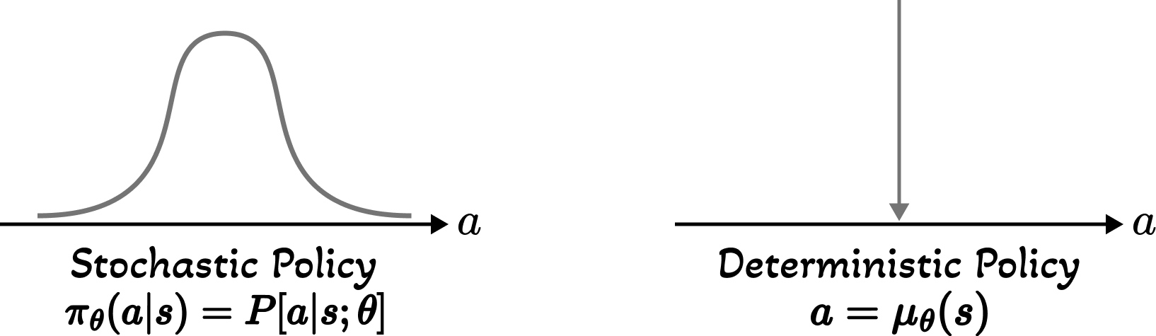
Policies can be either deterministic or stochastic. A deterministic policy $\mu: \mathcal{S} \rightarrow \mathcal{A}$ maps each state to a specific action, while a stochastic policy $\pi: \mathcal{S} \times \mathcal{A} \rightarrow [0,1]$ defines a probability distribution over actions for each state. See Figure 2 for an illustration.
정책은 결정론적 또는 확률적일 수 있습니다. 결정론적 정책 $\mu: \mathcal{S} \rightarrow \mathcal{A}$는 각 상태를 특정 행동에 매핑하는 반면, 확률적 정책 $\pi: \mathcal{S} \times \mathcal{A} \rightarrow [0,1]$은 각 상태에 대한 행동에 대한 확률 분포를 정의합니다. 그림 2를 참조하세요.
Policy Gradient 정책 그래디언트
Policy-based methods typically use policy gradient algorithms, which optimize the policy parameters by performing gradient ascent on the expected return:
정책 기반 방법은 일반적으로 정책 그래디언트 알고리즘을 사용하며, 이는 기대 수익에 대한 그래디언트 상승을 수행하여 정책 매개변수를 최적화합니다:
The parameters are updated using gradient ascent:
매개변수는 그래디언트 상승을 사용하여 업데이트됩니다:
Policy-based methods excel in: (1) continuous action spaces, (2) learning stochastic policies (useful for partially observable environments), and (3) scenarios where the optimal policy is simpler than the optimal value function. Examples include REINFORCE, PPO, and TRPO.
정책 기반 방법은 다음에서 뛰어납니다: (1) 연속 행동 공간, (2) 확률적 정책 학습 (부분 관측 가능 환경에 유용), (3) 최적 정책이 최적 가치 함수보다 간단한 시나리오. 예로는 REINFORCE, PPO, TRPO가 있습니다.
3.3 Model-Based RL 3.3 모델 기반 RL
Model-based methods explicitly learn a model of the environment's dynamics (transition function $P(s'|s,a)$ and reward function $R(s,a)$) and use this model for planning or to generate simulated experience for learning. This contrasts with model-free methods (value-based and policy-based) that learn directly from experience without building an explicit environment model.
모델 기반 방법은 환경의 동역학 모델(전이 함수 $P(s'|s,a)$와 보상 함수 $R(s,a)$)을 명시적으로 학습하고 이 모델을 계획이나 학습을 위한 시뮬레이션 경험 생성에 사용합니다. 이는 명시적인 환경 모델을 구축하지 않고 경험에서 직접 학습하는 모델 프리 방법(가치 기반 및 정책 기반)과 대조됩니다.
Learning the Model 모델 학습
The environment model is typically learned through supervised learning from collected transitions. Given a dataset $\mathcal{D} = \{(s_i, a_i, r_i, s'_i)\}$, we learn:
환경 모델은 일반적으로 수집된 전이로부터 지도학습을 통해 학습됩니다. 데이터셋 $\mathcal{D} = \{(s_i, a_i, r_i, s'_i)\}$가 주어지면, 다음을 학습합니다:
Planning with the Model 모델을 사용한 계획
Once we have a model, we can use it for:
모델을 얻으면 다음에 사용할 수 있습니다:
- Planning: Using dynamic programming or tree search (e.g., MCTS) to find optimal policies without additional environment interaction.
- 계획: 추가 환경 상호작용 없이 최적 정책을 찾기 위해 동적 프로그래밍 또는 트리 검색(예: MCTS) 사용.
- Simulation: Generating synthetic trajectories to augment real experience, improving sample efficiency.
- 시뮬레이션: 실제 경험을 증강하기 위해 합성 궤적 생성, 샘플 효율성 향상.
- Prediction: Anticipating future states and rewards to improve decision-making.
- 예측: 의사결정을 개선하기 위해 미래 상태 및 보상 예측.
Advantages: Better sample efficiency (fewer environment interactions needed),
ability to plan ahead, and transferability across tasks.
Challenges: Model errors can compound over long horizons (model bias),
and learning accurate models in complex environments can be difficult.
Examples: Dyna-Q, MBPO (Model-Based Policy Optimization), MuZero.
장점: 더 나은 샘플 효율성(더 적은 환경 상호작용 필요),
미래 계획 능력, 작업 간 전이 가능성.
문제: 모델 오류가 긴 시간 범위에 걸쳐 누적될 수 있음(모델 편향),
복잡한 환경에서 정확한 모델을 학습하기 어려울 수 있음.
예: Dyna-Q, MBPO (Model-Based Policy Optimization), MuZero.
4. Exploration-Exploitation Tradeoff 4. 탐색-활용 균형
One of the most fundamental challenges in reinforcement learning is the exploration-exploitation tradeoff: the agent must balance between exploiting its current knowledge to maximize immediate rewards and exploring new actions to potentially discover better strategies. This section covers various approaches to address this challenge.
강화학습의 가장 근본적인 도전 과제 중 하나는 탐색-활용 균형입니다: 에이전트는 즉각적인 보상을 최대화하기 위해 현재 지식을 활용하는 것과 잠재적으로 더 나은 전략을 발견하기 위해 새로운 행동을 탐색하는 것 사이에서 균형을 맞춰야 합니다. 이 섹션에서는 이 도전 과제를 해결하기 위한 다양한 접근법을 다룹니다.
4.1 Simple Heuristics 4.1 단순 휴리스틱
Greedy Policy 탐욕 정책
The simplest approach is the greedy policy, which always selects the action with the highest estimated value:
가장 간단한 접근법은 탐욕 정책으로, 항상 추정된 가치가 가장 높은 행동을 선택합니다:
While this maximizes immediate exploitation, it performs no exploration and may get stuck in suboptimal policies.
이는 즉각적인 활용을 최대화하지만 탐색을 수행하지 않아 차선의 정책에 갇힐 수 있습니다.
ε-Greedy Policy ε-탐욕 정책
The ε-greedy policy introduces exploration by selecting a random action with probability $\epsilon$ and the greedy action with probability $1-\epsilon$:
ε-탐욕 정책은 확률 $\epsilon$으로 무작위 행동을 선택하고 확률 $1-\epsilon$으로 탐욕 행동을 선택하여 탐색을 도입합니다:
εz-Greedy Policy εz-탐욕 정책
A variant called εz-greedy uses a state-dependent exploration rate, where $\epsilon_z = \epsilon / z(s)$ and $z(s)$ is the number of times state $s$ has been visited. This gradually reduces exploration as states become more familiar.
εz-탐욕이라는 변형은 상태 의존적 탐색 비율을 사용하며, $\epsilon_z = \epsilon / z(s)$이고 $z(s)$는 상태 $s$가 방문된 횟수입니다. 이는 상태가 익숙해짐에 따라 탐색을 점진적으로 줄입니다.
Boltzmann Exploration (Softmax) 볼츠만 탐색 (소프트맥스)
Boltzmann exploration uses a softmax distribution over action values, providing a more graded exploration strategy. Actions with higher values are more likely to be selected, but lower-valued actions still have non-zero probability:
볼츠만 탐색은 행동 가치에 대한 소프트맥스 분포를 사용하여 더 점진적인 탐색 전략을 제공합니다. 더 높은 가치를 가진 행동이 선택될 가능성이 더 높지만, 낮은 가치의 행동도 0이 아닌 확률을 가집니다:
where $\tau$ is the temperature parameter: high $\tau$ leads to more uniform exploration, while low $\tau$ approaches greedy behavior.
여기서 $\tau$는 온도 매개변수입니다: 높은 $\tau$는 더 균등한 탐색으로 이어지고, 낮은 $\tau$는 탐욕적 행동에 가까워집니다.
ε-Greedy: Simple to implement, uniform exploration over non-greedy actions,
clear exploitation-exploration split.
Boltzmann: Proportional exploration based on action values, smoother transition between
exploration and exploitation, requires tuning temperature $\tau$.
ε-탐욕: 구현이 간단, 비탐욕 행동에 대한 균일한 탐색,
활용-탐색 분할이 명확함.
볼츠만: 행동 가치에 기반한 비례적 탐색, 탐색과 활용 간의 더 부드러운 전환,
온도 $\tau$ 조정이 필요함.
4.2 Methods Based on the Belief State MDP 4.2 신념 상태 MDP 기반 방법
When uncertainty about the environment model is explicitly maintained as a belief state, we can formulate exploration as part of the optimal solution to a more complex MDP. These methods provide principled approaches to exploration by treating it as an optimization problem.
환경 모델에 대한 불확실성을 신념 상태로 명시적으로 유지할 때, 탐색을 더 복잡한 MDP의 최적 솔루션의 일부로 공식화할 수 있습니다. 이러한 방법은 탐색을 최적화 문제로 취급하여 원칙적인 접근법을 제공합니다.
Bandit Case: Gittins Indices 밴딧 경우: 기틴스 인덱스
For multi-armed bandit problems (single-state MDPs), the optimal exploration-exploitation strategy can be characterized by Gittins indices. Each action is assigned an index value that represents its attractiveness considering both immediate reward and information gain:
다중 암 밴딧 문제(단일 상태 MDP)의 경우, 최적 탐색-활용 전략은 기틴스 인덱스로 특성화될 수 있습니다. 각 행동에는 즉각적인 보상과 정보 이득을 모두 고려한 매력도를 나타내는 인덱스 값이 할당됩니다:
where $b$ is the belief state about the action's reward distribution, and $\tau$ is a stopping time. The optimal policy simply selects the action with the highest Gittins index at each time step.
여기서 $b$는 행동의 보상 분포에 대한 신념 상태이고, $\tau$는 정지 시간입니다. 최적 정책은 각 시간 단계에서 가장 높은 기틴스 인덱스를 가진 행동을 선택하기만 하면 됩니다.
MDP Case: Bayes-Adaptive MDPs (BAMDP) MDP 경우: 베이즈 적응 MDP (BAMDP)
For general MDPs with unknown dynamics, the problem can be formulated as a Bayes-Adaptive MDP. The augmented state space consists of the original state $s$ and a belief over the MDP parameters $b$:
동역학을 알 수 없는 일반 MDP의 경우, 문제를 베이즈 적응 MDP로 공식화할 수 있습니다. 확장된 상태 공간은 원래 상태 $s$와 MDP 매개변수에 대한 신념 $b$로 구성됩니다:
where $\Theta$ is the space of possible MDP parameters (transition and reward functions). The belief $b$ is updated via Bayesian inference as new transitions are observed:
여기서 $\Theta$는 가능한 MDP 매개변수(전이 및 보상 함수)의 공간입니다. 신념 $b$는 새로운 전이가 관찰됨에 따라 베이지안 추론을 통해 업데이트됩니다:
While BAMDP provides the theoretically optimal solution to exploration-exploitation, solving it exactly is computationally intractable for most problems. Approximate methods and heuristics inspired by this framework (like UCB and Thompson sampling) are more practical.
BAMDP는 탐색-활용에 대한 이론적으로 최적의 솔루션을 제공하지만, 대부분의 문제에 대해 정확하게 푸는 것은 계산적으로 불가능합니다. 이 프레임워크에서 영감을 받은 근사 방법과 휴리스틱(UCB 및 톰슨 샘플링 등)이 더 실용적입니다.
4.3 Upper Confidence Bounds (UCBs) 4.3 상한 신뢰 구간 (UCBs)
Basic Idea 기본 아이디어
The principle of optimism in the face of uncertainty guides UCB methods: assign each action an upper confidence bound on its value, then select the action with the highest bound. This naturally balances exploitation (actions with high estimated value) and exploration (actions with high uncertainty).
불확실성 하의 낙관주의 원칙이 UCB 방법을 안내합니다: 각 행동에 가치에 대한 상한 신뢰 구간을 할당한 다음, 가장 높은 구간을 가진 행동을 선택합니다. 이는 활용(높은 추정 가치를 가진 행동)과 탐색(높은 불확실성을 가진 행동) 사이의 균형을 자연스럽게 맞춥니다.
where $\hat{Q}(a)$ is the estimated value (exploitation term) and $U(a)$ is the uncertainty bonus (exploration term).
여기서 $\hat{Q}(a)$는 추정 가치(활용 항)이고 $U(a)$는 불확실성 보너스(탐색 항)입니다.
Bandit Case: Frequentist Approach 밴딧 경우: 빈도주의 접근
For multi-armed bandits, UCB algorithms use concentration inequalities like the Chernoff-Hoeffding inequality to bound the true value:
다중 암 밴딧의 경우, UCB 알고리즘은 체르노프-회프딩 부등식과 같은 집중 부등식을 사용하여 실제 가치를 제한합니다:
where $\hat{Q}_t(a)$ is the empirical mean reward for action $a$, $n_t(a)$ is the number of times action $a$ has been selected by time $t$. The famous UCB1 algorithm uses:
여기서 $\hat{Q}_t(a)$는 행동 $a$에 대한 경험적 평균 보상이고, $n_t(a)$는 시간 $t$까지 행동 $a$가 선택된 횟수입니다. 유명한 UCB1 알고리즘은 다음을 사용합니다:
where $c$ is an exploration constant (often $c = \sqrt{2}$). This achieves logarithmic regret: $O(\log T)$.
여기서 $c$는 탐색 상수입니다(종종 $c = \sqrt{2}$). 이는 대수적 후회를 달성합니다: $O(\log T)$.
Bandit Case: Bayesian Approach 밴딧 경우: 베이지안 접근
A Bayesian UCB approach maintains a posterior distribution over each action's value and selects based on upper quantiles of these posteriors:
베이지안 UCB 접근법은 각 행동의 가치에 대한 사후 분포를 유지하고 이러한 사후의 상위 분위수를 기반으로 선택합니다:
where $Q_{\alpha}^t(a)$ is the $(1-\alpha)$-quantile of the posterior distribution for action $a$ at time $t$. As more data is collected, the posterior concentrates and the quantile approaches the true mean.
여기서 $Q_{\alpha}^t(a)$는 시간 $t$에서 행동 $a$에 대한 사후 분포의 $(1-\alpha)$-분위수입니다. 더 많은 데이터가 수집됨에 따라 사후가 집중되고 분위수가 실제 평균에 접근합니다.
MDP Case MDP 경우
UCB principles extend to full MDPs through exploration bonuses added to the value function or Q-function. For example, the UCRL2 algorithm constructs confidence intervals around transition probabilities and rewards, then optimistically plans using the upper bounds:
UCB 원칙은 가치 함수 또는 Q-함수에 추가된 탐색 보너스를 통해 완전한 MDP로 확장됩니다. 예를 들어, UCRL2 알고리즘은 전이 확률과 보상 주위에 신뢰 구간을 구성한 다음 상한을 사용하여 낙관적으로 계획합니다:
where $\mathcal{M}(s)$ is the confidence set of plausible MDPs given observations. Modern deep RL methods incorporate exploration bonuses based on state visitation counts, prediction errors, or ensemble disagreement.
여기서 $\mathcal{M}(s)$는 관찰을 고려할 때 타당한 MDP의 신뢰 집합입니다. 현대 심층 RL 방법은 상태 방문 횟수, 예측 오류 또는 앙상블 불일치를 기반으로 한 탐색 보너스를 통합합니다.
UCB methods provide theoretical guarantees (logarithmic regret bounds), are parameter-free or require minimal tuning, and provide a principled exploration strategy that automatically adapts to uncertainty.
UCB 방법은 이론적 보장(대수적 후회 한계)을 제공하고, 매개변수가 없거나 최소한의 조정이 필요하며, 불확실성에 자동으로 적응하는 원칙적인 탐색 전략을 제공합니다.
4.4 Thompson Sampling 4.4 톰슨 샘플링
Thompson sampling (also called posterior sampling) is a Bayesian approach that naturally balances exploration and exploitation through randomization. Instead of selecting the action with the highest upper confidence bound, Thompson sampling:
톰슨 샘플링(사후 샘플링이라고도 함)은 무작위화를 통해 탐색과 활용의 균형을 자연스럽게 맞추는 베이지안 접근법입니다. 가장 높은 상한 신뢰 구간을 가진 행동을 선택하는 대신, 톰슨 샘플링은:
- Maintains a posterior distribution over the unknown parameters (e.g., reward distributions, value functions)
- 알 수 없는 매개변수에 대한 사후 분포를 유지합니다(예: 보상 분포, 가치 함수)
- Samples a parameter configuration from the posterior
- 사후에서 매개변수 구성을 샘플링합니다
- Acts optimally with respect to the sampled parameters
- 샘플링된 매개변수에 대해 최적으로 행동합니다
- Updates the posterior with new observations
- 새로운 관찰로 사후를 업데이트합니다
The key insight is that the probability of selecting an action is proportional to the probability that it is optimal given current beliefs. Actions that are likely to be optimal or very uncertain (and thus might be optimal) receive more exploration.
핵심 통찰은 행동을 선택할 확률이 현재 신념을 고려할 때 최적일 확률에 비례한다는 것입니다. 최적일 가능성이 높거나 매우 불확실한(따라서 최적일 수 있는) 행동은 더 많은 탐색을 받습니다.
Example: Bernoulli Bandits 예시: 베르누이 밴딧
For bandits with Bernoulli rewards, using a Beta prior $\text{Beta}(\alpha_a, \beta_a)$ for each action $a$ leads to a simple update rule. After observing reward $r \in \{0,1\}$:
베르누이 보상을 가진 밴딧의 경우, 각 행동 $a$에 대해 베타 사전 $\text{Beta}(\alpha_a, \beta_a)$를 사용하면 간단한 업데이트 규칙이 생성됩니다. 보상 $r \in \{0,1\}$을 관찰한 후:
Extension to MDPs MDP로의 확장
Thompson sampling extends to MDPs by maintaining posteriors over transition dynamics $P(s'|s,a)$ and reward functions $R(s,a)$. At each episode or planning step:
톰슨 샘플링은 전이 동역학 $P(s'|s,a)$와 보상 함수 $R(s,a)$에 대한 사후를 유지하여 MDP로 확장됩니다. 각 에피소드 또는 계획 단계에서:
- Sample an MDP from the posterior: $\tilde{M} \sim p(M | \mathcal{D})$
- 사후에서 MDP를 샘플링: $\tilde{M} \sim p(M | \mathcal{D})$
- Solve for the optimal policy in the sampled MDP: $\pi^* = \arg\max_{\pi} V_{\tilde{M}}^{\pi}$
- 샘플링된 MDP에서 최적 정책을 풀기: $\pi^* = \arg\max_{\pi} V_{\tilde{M}}^{\pi}$
- Execute the policy to collect new data
- 새로운 데이터를 수집하기 위해 정책을 실행
- Update the posterior with the new observations
- 새로운 관찰로 사후를 업데이트
Theoretical guarantees: Achieves logarithmic regret like UCB in many settings.
Computational efficiency: Often simpler to implement than computing confidence bounds.
Empirical performance: Frequently outperforms UCB in practice, especially in complex domains.
Natural handling of delayed rewards: The Bayesian framework naturally propagates uncertainty through time.
Examples: PSRL (Posterior Sampling for RL), RLSVI (RL with Randomized Value Functions).
이론적 보장: 많은 설정에서 UCB와 같은 대수적 후회를 달성합니다.
계산 효율성: 신뢰 구간을 계산하는 것보다 구현이 더 간단한 경우가 많습니다.
경험적 성능: 실제로 특히 복잡한 도메인에서 UCB보다 자주 더 나은 성능을 보입니다.
지연된 보상의 자연스러운 처리: 베이지안 프레임워크는 시간에 걸쳐 불확실성을 자연스럽게 전파합니다.
예: PSRL (RL을 위한 사후 샘플링), RLSVI (무작위 가치 함수를 사용한 RL).
5. Implementing RL with JAX 5. JAX로 RL 구현하기
Now that we've covered the theoretical foundations of reinforcement learning—from MDPs and value functions to exploration strategies—it's time to discuss how we can efficiently implement these algorithms in practice. In this course, we use JAX, a powerful numerical computing library that brings together the best features of NumPy, automatic differentiation, and high-performance compilation.
이제 MDP와 가치 함수부터 탐색 전략까지 강화학습의 이론적 기초를 다루었으므로, 이러한 알고리즘을 실제로 효율적으로 구현하는 방법에 대해 논의할 차례입니다. 이 과정에서는 NumPy의 장점, 자동 미분, 고성능 컴파일을 결합한 강력한 수치 계산 라이브러리인 JAX를 사용합니다.
Why JAX for Reinforcement Learning? 왜 강화학습에 JAX를 사용하는가?
JAX is particularly well-suited for RL research and implementation due to several key features that directly address the computational challenges we encounter in RL algorithms:
JAX는 RL 알고리즘에서 마주하는 계산적 도전 과제를 직접적으로 해결하는 여러 핵심 기능으로 인해 RL 연구 및 구현에 특히 적합합니다:
Key Advantages 주요 장점
| Feature특징 | Benefit for RLRL에 대한 이점 |
|---|---|
| JIT Compilation | Fast execution of iterative algorithms반복 알고리즘의 빠른 실행 |
| Automatic Differentiation | Easy implementation of gradient-based methods그래디언트 기반 방법의 쉬운 구현 |
| Vectorization (vmap) | Parallel environment simulation병렬 환경 시뮬레이션 |
| GPU/TPU Support | Scalable to large-scale problems대규모 문제로 확장 가능 |
| Functional Programming | Clean, composable algorithm implementations깔끔하고 조합 가능한 알고리즘 구현 |
Using JAX's vmap, we can vectorize our DP algorithms to solve multiple MDPs in parallel, achieving significant speedups for hyperparameter search or multi-task learning scenarios.
JAX의 vmap을 사용하면 DP 알고리즘을 벡터화하여 여러 MDP를 병렬로 해결할 수 있으며, 하이퍼파라미터 검색이나 멀티태스크 학습 시나리오에서 상당한 속도 향상을 달성할 수 있습니다.
6. Summary and Key Takeaways 6. 요약 및 핵심 사항
In this introductory week, we've laid the foundation for understanding reinforcement learning and its core principles. Let's recap the essential concepts we've covered:
이번 입문 주차에서 우리는 강화학습과 그 핵심 원리를 이해하기 위한 기초를 다졌습니다. 다룬 핵심 개념을 요약해보겠습니다:
Core Concepts 핵심 개념
RL is fundamentally about an agent learning to make optimal decisions through interaction with an environment. The agent observes states, takes actions according to its policy, and receives rewards. The goal is to maximize cumulative reward over time.
RL은 근본적으로 에이전트가 환경과의 상호작용을 통해 최적의 결정을 내리는 방법을 학습하는 것입니다. 에이전트는 상태를 관찰하고, 정책에 따라 행동을 취하며, 보상을 받습니다. 목표는 시간에 걸쳐 누적 보상을 최대화하는 것입니다.
We formalize RL problems using different frameworks: MDPs for fully observable environments with Markovian dynamics, POMDPs for partially observable settings where the agent must maintain belief states, and Contextual MDPs for problems with external context information.
RL 문제를 다양한 프레임워크로 공식화합니다: 마르코프 동역학을 가진 완전 관측 가능 환경을 위한 MDP, 에이전트가 신념 상태를 유지해야 하는 부분 관측 가능 설정을 위한 POMDP, 외부 맥락 정보가 있는 문제를 위한 맥락적 MDP.
Value-based methods learn value functions (V or Q) and derive policies from them using Bellman equations and TD learning. Policy-based methods directly optimize the policy using gradient ascent on expected returns. Model-based methods learn environment models and use them for planning or generating synthetic experience.
가치 기반 방법은 가치 함수(V 또는 Q)를 학습하고 벨만 방정식과 TD 학습을 사용하여 정책을 도출합니다. 정책 기반 방법은 기대 수익에 대한 그래디언트 상승을 사용하여 정책을 직접 최적화합니다. 모델 기반 방법은 환경 모델을 학습하고 계획이나 합성 경험 생성에 사용합니다.
The exploration-exploitation tradeoff is central to RL. We explored various strategies: simple heuristics like ε-greedy and Boltzmann exploration, principled approaches based on belief state MDPs (Gittins indices, BAMDPs), Upper Confidence Bounds with theoretical guarantees, and Thompson sampling which balances exploration naturally through Bayesian randomization.
탐색-활용 균형은 RL의 핵심입니다. 다양한 전략을 탐구했습니다: ε-탐욕과 볼츠만 탐색 같은 단순 휴리스틱, 신념 상태 MDP 기반의 원칙적 접근법(기틴스 인덱스, BAMDP), 이론적 보장을 가진 상한 신뢰 구간, 베이지안 무작위화를 통해 탐색의 균형을 자연스럽게 맞추는 톰슨 샘플링.
JAX provides the ideal framework for implementing RL algorithms efficiently: JIT compilation for speed, automatic differentiation for gradient-based methods, vectorization for parallel environments, and seamless GPU/TPU support for scalability.
JAX는 RL 알고리즘을 효율적으로 구현하기 위한 이상적인 프레임워크를 제공합니다: 속도를 위한 JIT 컴파일, 그래디언트 기반 방법을 위한 자동 미분, 병렬 환경을 위한 벡터화, 확장성을 위한 원활한 GPU/TPU 지원.
Looking Ahead 앞으로의 계획
With these foundational concepts in place, we're ready to dive into specific algorithms in the coming weeks. We'll start with classic methods like Q-learning and SARSA, move on to policy gradient methods like REINFORCE and Actor-Critic, and eventually explore modern deep RL algorithms like DQN, PPO, and beyond.
이러한 기초 개념을 갖추고, 앞으로 몇 주 동안 구체적인 알고리즘을 깊이 탐구할 준비가 되었습니다. Q-러닝과 SARSA 같은 고전적 방법으로 시작하여, REINFORCE와 액터-크리틱 같은 정책 그래디언트 방법으로 나아가고, 최종적으로 DQN, PPO 등 현대 심층 RL 알고리즘을 탐구할 것입니다.
Each algorithm will be accompanied by complete JAX implementations, mathematical derivations, and practical examples that you can run and experiment with. The goal is not just to understand the theory, but to develop intuition through hands-on coding and experimentation.
각 알고리즘에는 완전한 JAX 구현, 수학적 유도, 실행하고 실험할 수 있는 실용적인 예제가 함께 제공됩니다. 목표는 단순히 이론을 이해하는 것이 아니라, 직접 코딩하고 실험하면서 직관을 개발하는 것입니다.
Practice: Review the mathematical derivations and try implementing simple examples yourself.
Explore: Experiment with the JAX code examples and modify them to deepen your understanding.
Prepare: Make sure you're comfortable with the core concepts before moving to Week 2,
where we'll implement our first complete RL algorithm: Tabular Q-Learning.
연습: 수학적 유도를 복습하고 간단한 예제를 직접 구현해보세요.
탐구: JAX 코드 예제를 실험하고 수정하여 이해를 깊게 하세요.
준비: 2주차로 넘어가기 전에 핵심 개념을 편안하게 이해하도록 하세요.
2주차에서는 첫 번째 완전한 RL 알고리즘인 표 형식 Q-러닝을 구현할 것입니다.